Finite Element Analysis can generate stress contours within seconds. That speed often creates a dangerous illusion that a solved model is a reliable model. In reality, trustworthy engineering results are never produced in seconds. They are demonstrated through convergence.
Convergence in FEA is the mathematical and physical confirmation that a numerical solution is stable, consistent, and representative of real structural behaviour. Without convergence, an analysis is only a discretised approximation. With convergence, it becomes defensible engineering evidence.
This article explains convergence in FEA in depth, clarifies the difference between mesh convergence and nonlinear convergence, demonstrates how to perform a proper FEA convergence study, and addresses the critical issue of stress singularity in FEA. It also covers h-refinement versus p-refinement, energy-based accuracy assessment, and provides a practical checklist for validating FEA results before design approval.
What Is Convergence in FEA?
Convergence in FEA refers to the process by which the numerical solution approaches a stable value as the model is refined. In practical terms, convergence means that refining the mesh or reducing load increments does not significantly alter the results.
In linear analysis, convergence is primarily associated with mesh refinement. As the element size decreases, quantities such as stress and displacement should approach consistent values. If the solution continues to change significantly with further refinement, the model has not converged.
In nonlinear FEA analysis, convergence also refers to iterative equilibrium. Loads are applied incrementally, and at each step the solver balances external and internal forces. When the residual forces fall below tolerance, the iteration converges mathematically. However, mathematical convergence does not automatically guarantee physical correctness.
Mesh Convergence in FEA Analysis
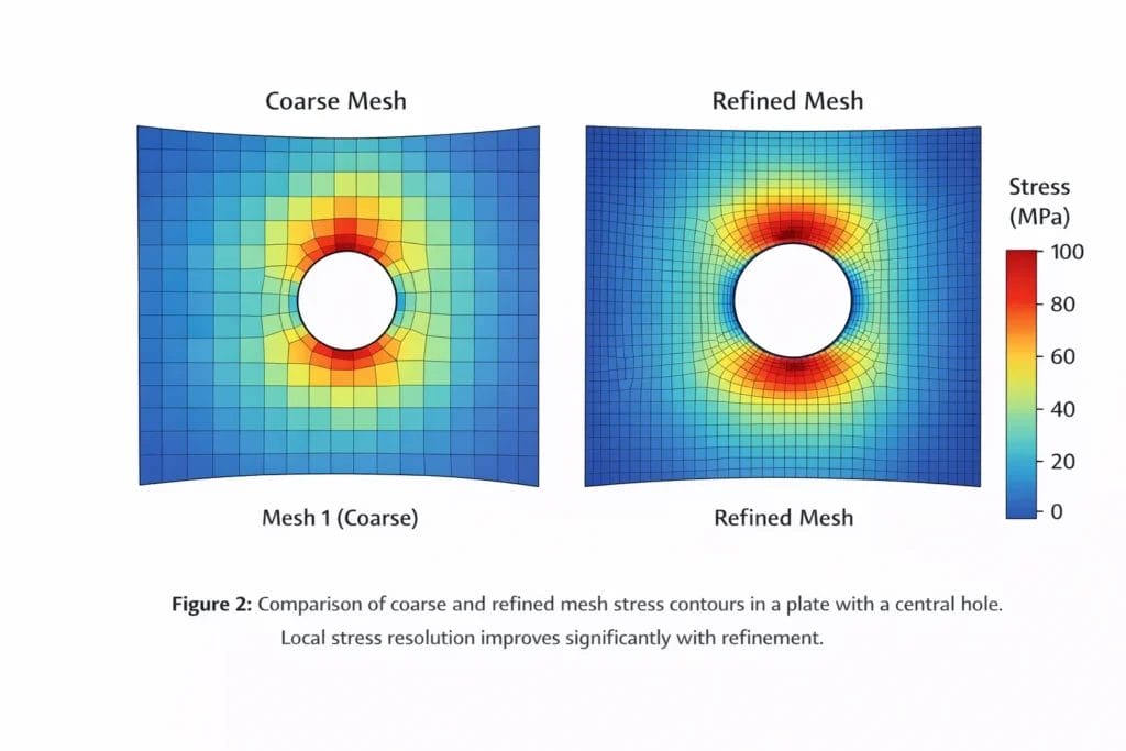
Every finite element model replaces a continuous structure with discrete elements. The mesh is therefore the bridge between physics and mathematics. If the discretisation is too coarse, stress gradients are poorly captured and peak values are underestimated. If it is excessively refined everywhere, computational cost increases dramatically and numerical artefacts may dominate localised regions.
Mesh convergence examines how sensitive results are to element size. As the mesh is refined, key quantities such as maximum stress, displacement, reaction forces, and strain energy should stabilise. When two successive refinements produce negligible variation typically within 2 to 5 percent per NAFEMS guidance the solution is considered mesh converged.
A proper FEA convergence study does not refine the entire model uniformly. Instead, refinement is applied in regions of high gradient: near stress concentrations, fillets, holes, contact interfaces, and load application zones. Refining low-gradient regions provides little benefit while dramatically increasing computation time. This principle is supported by Saint-Venant’s Principle, which states that stress disturbances introduced at a point decay rapidly with distance meaning remote regions require far less resolution than local stress concentration zones.
H-Refinement vs. P-Refinement
There are two fundamental strategies for improving mesh accuracy. Understanding the difference allows engineers to choose the most efficient approach for any given problem.
| Method | How It Works | Best Used When |
|---|---|---|
| h-Refinement | Reduces element size (increases element count) | Stress gradients, geometric complexity, contact zones |
| p-Refinement | Increases polynomial order of elements (higher-order shape functions) | Smooth solutions, bending-dominated problems, limited mesh density |
In h-refinement, the polynomial order of the element shape functions remains fixed while the element size is reduced. This is the most common approach and is well-suited to problems with localized stress gradients. In p-refinement, the mesh topology remains fixed while the polynomial order of the elements is increased, capturing more complex displacement fields within each element. Both methods can be combined in hp-refinement strategies for highly demanding problems.
How to Perform a Reliable FEA Convergence Study
A structured FEA convergence study follows a systematic refinement process. The model is first solved using a baseline mesh. Critical regions are then refined, and results are compared to the previous solution. The refinement process continues until key response variables stabilise.
The following example demonstrates convergence behaviour for a typical structural component under static loading. Maximum stress and displacement are recorded at each mesh refinement level:
| Mesh Level | Element Size | Max Stress (MPa) | Displacement (mm) | Change (%) |
|---|---|---|---|---|
| Mesh 1 — Coarse | 10 mm | 85 | 2.41 | — |
| Mesh 2 | 5 mm | 97 | 2.58 | 14.1% |
| Mesh 3 | 2.5 mm | 101 | 2.63 | 4.1% |
| Mesh 4 — Fine | 1.5 mm | 102 | 2.64 | 1.0% ✓ |
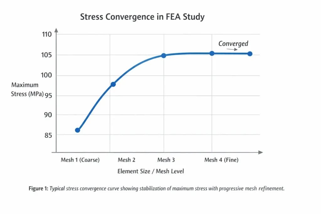
In this example, the solution is considered converged at Mesh 4, where the change in maximum stress drops below 2 percent. Note that displacement converges faster than stress a common characteristic of FEA, since displacements are primary unknowns and stresses are derived quantities with higher sensitivity to discretisation error.
Convergence Criterion: Per DNVGL-RP-F112 Appendix A.1, linear analysis convergence is confirmed when peak stress changes by less than 3% upon having local element size. For nonlinear analysis, the criterion applies to total strain energy (≤5%).
However, if peak stress increases continuously with refinement and does not stabilize, the model likely contains a stress singularity or an unrealistic constraint a situation addressed in detail in the next section.
Stress Singularity in FEA
Stress singularity in FEA is one of the most misunderstood sources of apparent non-convergence. Singularities occur at sharp internal corners, point loads, perfectly fixed constraints, or crack tips. In such cases, the theoretical stress approaches infinity. As the mesh is refined, the computed peak stress continues to increase without stabilising.
This behaviour does not indicate material failure. It indicates a mathematical artefact introduced by the idealisation of geometry or boundary conditions.
Identifying a Singularity vs a True Stress Concentration
- A real stress concentration caused by a fillet radius or a hole in a plate will produce a stress peak that stabilizes under mesh refinement. The stress is high but finite and physically meaningful.
- A singularity will not stabilize. Each successive refinement produces a higher peak stress without convergence. The location is always a geometric idealization a perfectly sharp re-entrant corner, a point load, or a fully fixed node.
How to Handle Singularities
- Averaged nodal stresses or stress linearisation methods must be used instead of peak nodal values in singular regions.
- Where possible, introduce a small fillet radius to replace the idealised sharp corner and restore physical realism.
- Alternatively, use submodelling extract boundary conditions from the global model and apply them to a refined local model with realistic geometry.
- For crack tip singularities, use dedicated fracture mechanics elements or contour integral methods rather than standard mesh refinement.
Failure to recognise stress singularity in FEA can lead to unnecessary redesign, incorrect safety factor assessment, or misidentified failure modes.
Nonlinear Convergence in FEA Analysis
In nonlinear analysis, convergence has an additional meaning. When material nonlinearity, large deformation, or contact behavior is present, the stiffness of the system evolves as loads are applied. The solver applies loads incrementally and performs iterative corrections typically using Newton-Raphson iteration until equilibrium is achieved.
Convergence is reached when residual forces fall below defined tolerances. If convergence fails, it may indicate excessive load increments, unstable contact conditions, inadequate boundary conditions, or true structural instability.
Temporal Convergence in Dynamic Analysis
In transient, dynamic, and vibration analyses, there is a third dimension of convergence: temporal convergence. The time step size must be small enough that the numerical integration scheme accurately captures the system’s dynamic response. If the time step is too large, the solution may appear to converge at each step while still misrepresenting the overall dynamic behaviour.
As with spatial mesh refinement, temporal convergence is confirmed by progressively reducing the time step size and observing whether key response quantities peak displacement, acceleration, or stress stabilize. Temporal and spatial convergence must be demonstrated independently.
Nonlinear convergence confirms force equilibrium, not accuracy. A model can converge numerically while still being physically incorrect due to improper boundary conditions or unrealistic stiffness assumptions.
The Hidden Risk of False Convergence
A model may appear stable under mesh refinement and satisfy solver residual criteria while still misrepresenting physical behaviour. This phenomenon is often referred to as false convergence. False convergence commonly arises when boundary conditions are over-constrained, contact stiffness is artificially high, or local mesh refinement is neglected near stress gradients. The solver may report successful convergence, yet the stress distribution is physically unrealistic.
Common Causes of False Convergence
- Over-constrained boundary conditions that artificially stiffen the model, suppressing realistic deformation
- Contact stiffness values set too high, preventing natural interface behaviour
- Insufficient mesh density in stress gradient zones, causing smooth but inaccurate stress distributions
- Inappropriate material models that artificially limit plastic flow or damage progression
Therefore, convergence must always be accompanied by engineering judgement. Deformation patterns must follow logical load paths. Reaction forces must balance applied loads. Energy trends must stabilize consistently.
Energy-Based Accuracy Assessment
Peak stress comparison alone is often insufficient for evaluating convergence quality. Strain energy provides a more stable global metric. As the mesh is refined, total strain energy should approach a constant value.
Energy norm error estimates are frequently more reliable indicators of global solution accuracy than localized stress peaks. This is because strain energy is a volume-integrated quantity it averages behavior across the entire model making it far less sensitive to local mesh deficiencies than point-wise stress values.
If strain energy stabilises while peak stress fluctuates slightly in regions without singularities, the solution may still be considered sufficiently accurate for design purposes. Conversely, if strain energy continues to change significantly between refinements, global discretisation error remains unacceptably high regardless of localised stress stability.
How to Validate FEA Results Before Design Approval
Validating FEA results requires more than observing convergence trends. Before approving a design based on simulation, engineers must complete a structured set of checks that confirm the model is physically realistic, numerically stable, and defensible under audit or failure investigation.
The following checklist consolidates best-practice validation requirements for both linear and nonlinear FEA:
| # | Validation Requirement | Technical Verification Method | Acceptance Criteria / Evidence |
|---|---|---|---|
| 1 | Mesh Convergence Demonstrated | Minimum 3 systematic refinement levels in critical regions | Peak stress variation ≤ 3% (linear) or strain energy variation ≤ 5% (nonlinear) upon halving element size |
| 2 | Global Force Equilibrium Verified | Sum of reaction forces vs. applied loads | Imbalance ≤ 1% of total applied load |
| 3 | Moment Equilibrium Verified (if applicable) | Check reaction moments vs applied moments | Rotational equilibrium satisfied within solver tolerance |
| 4 | Energy Balance Consistency | Compare internal strain energy vs external work | Stable trend across refinements; no unexplained energy growth |
| 5 | Residual Convergence Confirmed (Nonlinear) | Review residual force and displacement plots per load step | Residuals reduced below solver-defined tolerance without oscillatory divergence |
| 6 | Contact Behaviour Validated (if applicable) | Check penetration, contact pressure distribution | Penetration within defined tolerance; no artificial stiffness spikes |
| 7 | Boundary Conditions Physically Justified | Engineering review of constraint assumptions | No artificial over-constraint or unintended load paths |
| 8 | Averaged vs Unaveraged Stress Compared | Inspect nodal stress smoothing effects | Large discrepancy investigated; singularities identified |
| 9 | Stress Singularities Identified and Classified | Monitor peak stress trend under refinement | Non-stabilising peaks treated as singularities; excluded from failure assessment |
| 10 | Deformation Pattern Physically Logical | Visual deformation review with scaled displacement | Load path consistent with structural mechanics principles |
| 11 | Material Model Appropriateness Verified | Review constitutive model vs real material behaviour | Correct yield criteria, hardening law, and strain limits applied |
| 12 | Sensitivity to Boundary Condition Variations Checked | Slight perturbation of constraints or load positions | No disproportionate stress amplification |
| 13 | Element Quality Metrics Reviewed | Aspect ratio, skewness, Jacobian check | All elements within solver-recommended quality limits |
| 14 | Submodelling or Local Refinement Applied Where Necessary | Extract refined model for high-gradient regions | Local solution consistent with global boundary conditions |
| 15 | Code Compliance Stress Categorisation (if applicable) | Linearisation of membrane + bending stress (ASME / DNV / FKM) | Stress components within allowable limits per governing code |
| 16 | Hand Calculation / Benchmark Correlation Performed | Compare with simplified analytical solution | Results within acceptable engineering deviation |
| 17 | Temporal Convergence Verified (Dynamic Analysis) | Reduce time step and compare response metrics | Peak response variation negligible with reduced time increment |
| 18 | Documentation Complete for Audit Traceability | Archive mesh levels, solver settings, assumptions | Full reproducibility of model and convergence evidence |
In nonlinear problems, residual force plots must confirm stable convergence at each load step. Deformation patterns must align with expected physical behavior. Contact penetrations must remain within acceptable tolerances. Where possible, results should be cross-checked against hand calculations for simplified load cases, experimental data, or published benchmark solutions.
Audit Standard: Without documented convergence and validation checks, simulation results cannot be considered defensible in regulatory audit, failure investigation, or design certification scenarios.
When Is a Coarse Mesh Acceptable?
Not every engineering decision requires highly refined meshes. Early-stage feasibility studies, stiffness comparisons, and conceptual evaluations may tolerate coarser discretisation. However, final design approval demands refinement in critical zones and documented convergence studies.
The required level of refinement is determined by risk, safety factors, and consequence of failure not by software capability alone. A coarse mesh used knowingly, with documented awareness of its limitations, is an engineering decision. A coarse mesh trusted blindly is an engineering risk.
Final Perspective
Convergence in FEA is not a software checkbox. It is evidence that the numerical approximation has approached physical reality.
Mesh convergence ensures that discretisation error is controlled. Nonlinear convergence confirms equilibrium. Temporal convergence validates dynamic accuracy. Stress singularity recognition prevents misinterpretation of infinite stresses. Energy stabilisation reinforces global accuracy. And a structured validation checklist transforms simulation output into defensible engineering evidence.
When these elements are demonstrated together and documented together simulation transitions from visualization to validation.
Written By

PANDHARINATH SANAP
CEO and Co-Founder | IntPE
Pandharinath Sanap is the CEO and Co-Founder of Ideametrics, with more than 15 years of experience in mechanical engineering, engineering assessments, and technical reviews across industrial projects. He is an International Professional Engineer (IntPE)… Know more