Computational Fluid Dynamics (CFD) is one of the most powerful tools in modern engineering. It allows engineers to simulate fluid flow, heat transfer, pressure distribution, and turbulence inside complex systems without building a physical prototype. From aircraft wings to industrial heat exchangers, CFD accelerates design cycles and lowers development cost.
Yet any experienced engineer will acknowledge: CFD is not a crystal ball. Simulation results sometimes diverge from experimental data, field measurements, or real-world performance. When that happens, trust in the simulation erodes—and engineering decisions become unreliable.
Understanding why CFD results differ from reality is not just an academic exercise. It is the foundation of responsible engineering simulation practice.
Why do CFD results differ from reality?
CFD simulations diverge from real-world behavior primarily because of modeling assumptions, mesh limitations, incorrect boundary conditions, turbulence model approximations, and insufficient experimental validation. Every simulation simplifies reality to make computation feasible and each simplification introduces potential error. Minimizing these gaps requires rigorous verification, validation, and engineering judgement.
What is CFD Simulation?
Computational Fluid Dynamics (CFD) is the use of numerical methods and algorithms to solve and analyse problems involving fluid flow. It simulates how gases and liquids move, interact with surfaces, exchange heat, and respond to applied forces.
At its core, CFD solves the Navier-Stokes equations a set of partial differential equations that govern conservation of mass, momentum, and energy in a fluid. These equations are highly nonlinear and cannot be solved analytically for most engineering problems. CFD discretizes the fluid domain into a computational mesh of millions of small cells and solves the governing equations numerically at each cell.
What CFD Predicts
- Velocity fields – how fast and in what direction fluid moves throughout the domain
- Pressure distribution – forces acting on surfaces and pressure losses through the system
- Turbulence intensity – chaotic fluctuations in flow velocity and direction
- Heat transfer – conduction, convection, and temperature gradient distribution
- Species concentration – mixing of different fluids or chemical species
CFD is a numerical approximation of physical flow behavior, not an exact replica. Every simulation makes assumptions, and the accuracy of results depends directly on the quality of those assumptions, the mesh, and the boundary conditions applied.
How Accurate is CFD Simulation?
CFD can achieve high accuracy, often within 2 to 10 percent of experimental results, when physics are modeled correctly, the mesh is sufficiently refined, and boundary conditions are realistic. In well-validated applications, such as external aerodynamics of streamlined bodies or fully developed pipe flow, CFD is a dependable engineering tool.
However, accuracy is not guaranteed. It depends on three pillars: physics modeling fidelity, numerical method quality, and systematic validation against physical experiments. Without all three, simulation results should be treated with caution.
Featured Snippet: CFD simulation accuracy typically ranges from 2 to 15 percent error compared to experimental data, depending on flow complexity and modeling choices. Simple, well-studied flows can achieve below 5 percent error. Complex turbulent, multiphase, or reactive flows carry higher uncertainty without careful model selection and thorough experimental validation.
Major Reasons CFD Results Differ From Reality
The following sections address the most common and consequential sources of discrepancy between CFD predictions and physical measurements.
1. Modeling Assumptions and Simplifications
Every CFD simulation begins with engineering assumptions that define what physics will be modeled, and what will be ignored. These assumptions are necessary to make computation tractable, but each introduces potential deviation from reality.
Steady vs. transient flow: Many simulations assume steady-state flow to save computational cost. Real flows are often unsteady vortex shedding, pulsating inlets, and time varying boundary conditions are transient phenomena that steady simulations cannot capture.
Incompressible vs. compressible flow: Assuming incompressibility is valid at low Mach numbers (below approximately 0.3), but at higher speeds, density changes significantly affect velocity and pressure fields. Applying incompressible solvers to high-speed flows introduces systematic error.
Symmetry assumptions: Simulating only half or a quarter of a geometry using symmetry planes is computationally efficient, but real flows are often asymmetric due to manufacturing tolerances, upstream disturbances, or turbulent fluctuations.
Simplified geometry: CFD models frequently omit small features such as fasteners, weld seams, surface roughness, or assembly gaps. These simplifications can meaningfully affect local flow behavior, especially in confined passages.
2. Mesh Quality and Grid Dependency
The computational mesh is the foundation of every CFD simulation. Poor mesh quality directly degrades result accuracy, regardless of how sophisticated the solver or turbulence model may be.
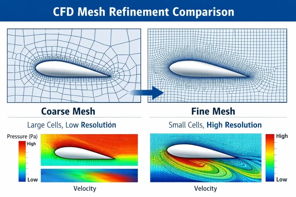
Figure 1: CFD mesh refinement comparison showing coarse mesh vs fine mesh resolution around an aerodynamic surface.
Coarse mesh resolution: Insufficient cell density fails to resolve steep gradients in velocity and pressure, particularly in regions of separation, recirculation, or jet impingement.
High skewness and poor aspect ratio: Highly distorted cells introduce numerical diffusion errors that smear flow features and produce inaccurate force predictions.
Insufficient near-wall cells: Wall boundary layers require very fine mesh resolution near solid surfaces, characterized by appropriate y+ values. Without adequate near-wall resolution, wall shear stress and heat transfer predictions become unreliable.
Mesh independence studies are essential: engineers must systematically refine the mesh and monitor key output quantities until results no longer change with further refinement. Results that have not passed this test should not be used for engineering decisions.
3. Incorrect Boundary Conditions
Boundary conditions define the environment surrounding the simulation domain and control the entire solution. Errors in boundary conditions propagate through every cell in the domain.
- Wrong inlet velocity profile – specifying uniform inflow when the real flow has a developed turbulent profile
- Unrealistic turbulence intensity – using default values (5 percent) when actual intensity may be 15 to 20 percent in industrial equipment
- Incorrect outlet pressure – assuming zero gauge pressure when downstream backpressure exists
- Wrong thermal boundary conditions – specifying constant wall temperature when the actual condition is convective heat flux
Even a well-constructed mesh and accurate turbulence model cannot compensate for incorrect boundary conditions. Engineers must characterize real operating conditions through physical measurements or validated empirical data before defining simulation boundaries.
4. Turbulence Model Limitations
Turbulence is one of the most complex phenomena in fluid mechanics—and the largest single source of modelling uncertainty in most industrial CFD simulations.
RANS models (k-epsilon, k-omega SST): Reynolds-Averaged Navier-Stokes models solve for time-averaged flow and model all turbulence with empirical closures. They are computationally efficient but rely on calibration constants that may not generalize across all flow regimes. k-epsilon performs well in free-stream flows but struggles with adverse pressure gradients. k-omega SST is more robust near walls but sensitive to freestream turbulence specification.
LES (Large Eddy Simulation): Resolves large turbulent structures directly and models only small scales. Far more accurate for separated and highly unsteady flows, but requires very fine mesh and is computationally 10 to 100 times more expensive than RANS.
DNS (Direct Numerical Simulation): Resolves all scales of turbulence with no modelling whatsoever. Extremely accurate but computationally prohibitive for all but simple, low Reynolds number academic flows.
No turbulence model is universally correct. Engineers must select the appropriate model for their specific flow regime, understand its known limitations, and validate predictions against experimental turbulence data where possible.
5. Numerical Errors and Solver Limitations
Even when physics and geometry are correctly defined, numerical solution methods introduce their own errors.
Discretization errors: Converting continuous differential equations into discrete algebraic equations on a mesh introduces truncation errors that depend on mesh size and the order of the numerical scheme.
Convergence errors: Iterative solvers may be stopped before achieving full convergence. Poorly converged solutions can appear visually smooth while containing significant residual imbalances in mass or momentum.
Round-off errors: Floating-point arithmetic accumulates small errors, especially in long transient runs or poorly conditioned linear systems. Double precision arithmetic mitigates but does not eliminate this issue.
Solver instability: Aggressive relaxation factors, excessive time steps, or poor initial conditions can drive iterative solvers to diverge or oscillate, producing unphysical results.
6. Geometry and Manufacturing Differences
The CFD model geometry is almost always an idealized version of physical hardware. Real manufactured parts deviate from design intent in ways that can significantly affect flow behaviour.
- Surface roughness – even machined surfaces have Ra values that alter boundary layer transition and wall friction
- Manufacturing tolerances – gaps, misalignments, and dimensional deviations change local flow resistance
- Corrosion and deposits – scale buildup in heat exchangers, fouling in pipes, and oxidation on turbine blades modify effective geometry over time
- Assembly distortions – bolted flanges, welded joints, and gasket compression alter local clearances from the nominal design
Engineers must assess whether geometric deviations are significant for their application and, where appropriate, include surface roughness models or geometric perturbation studies in their simulation workflow.
7. Lack of Experimental Validation
Perhaps the most critical, and most frequently overlooked, source of CFD unreliability is insufficient validation against physical data. Completing a simulation and obtaining results is not the same as knowing those results are correct.
Experimental validation methods for CFD include:
- Wind tunnel testing with pressure taps, hot-wire anemometry, and aerodynamic force balances
- Particle Image Velocimetry (PIV) for full-field velocity measurements without flow intrusion
- Pressure transducer arrays in pipe, duct, and manifold systems
- Thermocouple or infrared thermography for thermal validation
- Field measurements from installed equipment using flow meters and performance data
Engineering correlation, systematically comparing CFD predictions to measurements across a range of operating conditions, builds confidence that the simulation captures the underlying physics correctly. A validated model can then be used predictively within its established operating envelope.
CFD Verification vs Validation
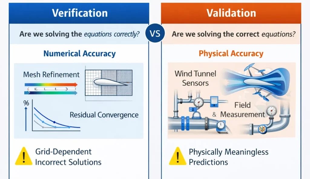
Figure 2: CFD Verification vs Validation in Engineering Simulations.
These two concepts are frequently confused but represent fundamentally different quality assurance activities in simulation engineering.
Verification asks: ‘Are we solving the equations correctly?’ It confirms that the numerical implementation is mathematically sound, that the discretized equations converge to the exact solution of the governing equations as mesh and time step are refined.
Validation asks: ‘Are we solving the correct equations?’ It confirms that the mathematical model, including turbulence models, boundary conditions, and physical assumptions, accurately represents the real physical phenomenon being studied.
A CFD solution can be fully verified (mathematically correct) yet invalid (physically wrong) if the wrong model was selected. Both activities are required for credible simulation practice.
| Aspect | Verification | Validation |
|---|---|---|
| Question | Are we solving the equations correctly? | Are we solving the right equations? |
| Focus | Numerical accuracy | Physical accuracy |
| Methods | Mesh convergence, residual checks | Wind tunnel, field measurement |
| Risk if skipped | Grid-dependent, incorrect solutions | Physically meaningless predictions |
How Engineers Improve CFD Accuracy
Professional simulation engineers follow a systematic workflow to maximize result reliability. These best practices are standard in high-quality CFD engineering work.
Mesh Independence Studies: Systematically refine the mesh in at least three successive levels. Monitor key output quantities at each level and report the mesh density at which results converge. First-attempt mesh results should never be accepted without this check.
Sensitivity Analysis: Vary key modeling inputs, turbulence intensity, inlet velocity profile, wall roughness height, and quantify how output predictions respond. High sensitivity signals a need for better-characterized input data.
Turbulence Model Comparison: Run the same case with multiple turbulence models. Assess which model produces results most consistent with available validation data or empirical correlations for that flow regime.
Realistic Boundary Conditions: Wherever possible, derive inlet conditions from measurements, velocity profiles from Pitot traverses, turbulence intensity from hot-wire surveys, or temperature profiles from thermocouple arrays.
Experimental Validation: Validate at least one operating condition against physical measurements before using the model predictively. Extend validation to multiple operating points when the design space is broad.
The most credible engineering outcomes combine simulation, sensitivity analysis, turbulence model comparison, and experimental correlation. Simulation accelerates design exploration; physical testing confirms the model is trustworthy.
Real Engineering Example: Pump Impeller Simulation
Consider a centrifugal pump impeller designed for a water treatment application. A steady-state RANS CFD simulation predicted hydraulic efficiency of 88 percent at the design flow rate, well within the project target.
During factory acceptance testing, the physical pump achieved only 81 percent hydraulic efficiency. The 7-point discrepancy triggered a detailed engineering investigation.
Post-test analysis identified two root causes:
- The CFD model used a uniform inlet velocity profile, while the actual installation had a 90-degree elbow immediately upstream that generated a swirling, asymmetric inlet flow.
- The steady-state RANS model did not resolve periodic rotor-stator interaction effects, which caused unsteady recirculation losses at the impeller leading edge that the time-averaged simulation missed entirely.
Engineers corrected the model by: (1) extending the inlet domain to include the upstream elbow, allowing the swirl profile to develop physically; (2) switching to an unsteady RANS approach to resolve rotor-stator interaction losses; and (3) incorporating turbulence intensity values measured at the physical inlet flange.
The corrected simulation predicted 82 percent efficiency, within 1.2 percent of the measured value. The validated model was then used confidently to optimize impeller blade geometry for a redesigned pump configuration.
This example demonstrates that CFD discrepancies are diagnosable and correctable, but only when engineers commit to rigorous validation and are willing to revisit modeling assumptions when experimental data reveals inconsistencies.
Key Takeaways
- CFD is a powerful approximation tool, not an exact physical replica, every simulation makes simplifying assumptions that introduce potential error.
- The most common sources of CFD inaccuracy are turbulence model limitations, incorrect boundary conditions, insufficient mesh resolution, and geometric simplifications.
- Mesh independence studies are non-negotiable: results that have not been tested for grid dependency should not inform engineering decisions.
- Boundary conditions must reflect real operating conditions, default or assumed values frequently introduce systematic, correctable bias.
- Verification confirms mathematical correctness; validation confirms physical accuracy, both are required for credible simulation practice.
- Experimental validation is not optional: at least one operating condition should be confirmed against physical measurements before the model is used predictively.
- Professional CFD practice combines simulation, sensitivity analysis, turbulence model comparison, and experimental correlation to deliver trustworthy engineering results.
Frequently Asked Questions
CFD simulations differ from experiments because of modeling assumptions, turbulence model approximations, incorrect boundary conditions, insufficient mesh resolution, and geometric simplifications. Real physical systems also include surface roughness, manufacturing tolerances, and installation effects that are typically absent from simulation models.
CFD simulation accuracy typically ranges from 2 to 15 percent error relative to experimental data, depending on flow complexity and model selection. Well-validated simulations of simple geometries can achieve below 5 percent error. Complex turbulent or multiphase flows require careful model selection and thorough validation to achieve acceptable accuracy.
CFD errors arise from turbulence model limitations, numerical discretization, mesh quality deficiencies, incorrect boundary conditions, and geometry simplifications. Convergence errors from prematurely stopped iterative solvers and inadequate near-wall mesh resolution are also frequent contributors to inaccurate predictions.
Engineers validate CFD models by comparing simulation predictions to experimental measurements including wind tunnel data, pressure transducer readings, PIV velocity field data, flow meter measurements, and thermal surveys. Validation should span multiple operating conditions and be completed before the model is used to guide design decisions.
Written By

PANDHARINATH SANAP
CEO and Co-Founder | IntPE
Pandharinath Sanap is the CEO and Co-Founder of Ideametrics, with more than 15 years of experience in mechanical engineering, engineering assessments, and technical reviews across industrial projects. He is an International Professional Engineer (IntPE)… Know more